Package mogptk
MOGPTK is a Python toolkit for multi output Gaussian processes. It contains data handling classes and different multi output models to facilitate the training and prediction of multi channel data sets. It provides a complete toolkit to improve the training of MOGPs, where it allows for easy detrending or transformation of the data (such as taking the natural logarithm), functions that aid in adding gaps to the data or specifying which range should be predicted, and more.
The following four MOGP models have been implemented:
- Multi Output Spectral Mixture (MOSM) as proposed by [1]
- Cross Spectral Mixture (CSM) as proposed by [2]
- Convolutional Gaussian (CONV) as proposed by [3]
- Spectral Mixture - Linear Model of Coregionalization (SM-LMC) as proposed by combining SM [4] and LMC [5]
Each model has specialized methods for parameter estimation to improve training. For example, the MOSM model can estimate its parameters using the training of spectral mixture kernels for each of the channels individually. It can also estimate its parameters using Bayesian Nonparametric Spectral Estimation (BNSE) [6]. After parameter estimation, the training of the model will converge more rapidly and there is a higher chance it will converge at all. Additionally, some models allow the interpretation of the parameters by investigating the cross-correlation parameters between the channels to better interpret what the learned parameters actually mean.
- [1] G. Parra and F. Tobar, "Spectral Mixture Kernels for Multi-Output Gaussian Processes", Advances in Neural Information Processing Systems 31, 2017
- [2] K.R. Ulrich et al, "GP Kernels for Cross-Spectrum Analysis", Advances in Neural Information Processing Systems 28, 2015
- [3] M.A. Álvarez and N.D. Lawrence, "Sparse Convolved Multiple Output Gaussian Processes", Advances in Neural Information Processing Systems 21, 2009
- [4] A.G. Wilson and R.P. Adams, "Gaussian Process Kernels for Pattern Discovery and Extrapolation", International Conference on Machine Learning 30, 2013
- [5] P. Goovaerts, "Geostatistics for Natural Resource Evaluation", Oxford University Press, 1997
- [6] F. Tobar, "Bayesian Nonparametric Spectral Estimation", Advances in Neural Information Processing Systems 32, 2018
Installation
Make sure you have at least Python 3.6 and pip installed, and run the following command:
pip install mogptk
Glossary
- GP: Gaussian process, see Gaussian Processes for Machine Learning by C.E. Rasmussen and C.K.I. Williams.
- MOSM: Multi-output spectral mixture kernel, see Spectral Mixture Kernels for Multi-Output Gaussian Processes by G. Parra and F. Tobar.
- CSM: Cross spectral mixture kernel, see GP Kernels for Cross-Spectrum Analysis by K.R. Ulrich et al.
- CONV: Convolution Gaussian kernel, see Sparse Convolved Multiple Output Gaussian Processes by M.A. Álvarez and N.D. Lawrence.
- SM-LMC: Spectral mixture linear model of coregionalization kernel, see Gaussian Process Kernels for Pattern Discovery and Extrapolation by A.G. Wilson and R.P. Adams and the book "Geostatistics for Natural Resource Evaluation" by P. Goovaerts.
- M: the number of channels (i.e. output dimensions)
- N: the number of data points
- Q: the number of components to use for a kernel. Each component is added additively to the main kernel
Using the GPU
If a GPU is available through CUDA it will be automatically used in tensor calculations and may speed up training significantly. To get more information about whether CUDA is supported or which GPU is used, as well as more control over which CPU or GPU to use, see mogptk.gpr.config. For example, you can force CPU or GPU training:
mogptk.gpr.use_cpu(0)  # use the first CPU

mogptk.gpr.use_gpu(1)  # use the second GPU

mogptk.gpr.use_single_precision()  # higher performance and lower energy usage

mogptk.gpr.use_half_precision()  # even higher performance and lower energy usage
Advice on training
Training is not converging
This could be a host of causes, including:
- Data can not be fitted by kernel
-
- Did you remove the bias? Either set
data.transform(mogptk.TransformDetrend(degree=1))or add a mean function to the model
- Did you remove the bias? Either set
-
- Range of X axis may be very large, causing the kernel parameters to be orders of magnitude off their optimum
-
- Kernel does not fit the data, i.e. change the kernel
-
- Add more components to mixture kernels
- Kernel parameters are not properly initialized and training is stuck in a local minimum
- High learning rate, e.g. set
model.train(..., lr=0.1, ...) - Low learning rate or low amount of iterations
Loss over iterations has big jumps
The default learning rate for LBFGS is 1.0 and for Adam 0.001. Indications that your learning rate may be too high can be visualized after training by calling
model.plot_losses()
which will show the loss over iterations. When big jumps occur, especially upwards, you should probably lower your learning rate.
model.train('lbfgs', iters=500, lr=0.01)
Slow training performance
There are many ways to speed up the training of Gaussian processes, but we can divide the solutions into two groups: technical and theoretical solutions.
Technical
- Use a bigger computer
- Use less data points for training with
data.remove_randomly(pct=0.5) - Use a simpler kernel with less parameters (e.g. less mixture components)
- Use the GPU instead of the CPU with
mogptk.gpr.use_gpu() - Use lower precision such as
mogptk.gpr.use_single_precision()ormogptk.gpr.use_half_precision()
Theoretical
- Use a sparse model such as
mogptk.Titsias(inducing_points=20)with 20 inducing points and pass it to the model asinference - Use stochastic gradient descent as `mogptk.train(method='SGD') (WIP)
Mixture kernels have equal parameter values
When all subkernels of a mixture kernel are initialized with the same parameter values, training for each mixture kernel will perform similarly. This results in equal parameters values after optimization. To fix this, you should initialize parameter values, for example
Q = 10
input_dims = 1
kernel = mogptk.gpr.MixtureKernel(mogptk.gpr.SquaredExponentialKernel(), Q=Q)
for i in range(Q):
    kernel[i].magnitude.assign(torch.rand(1))
    kernel[i].lengthscale.assign(torch.rand(input_dims))
Unstable training: NaNs and Infs
Due to numerical issues this is unfortunately quite frequent in Gaussian process optimization, but there are several ways to mitigate this:
- Increase the jitter with mogptk.gpr.Kernel(..., jitter=1e-3), be aware that the jitter is multiplied by the average value on the diagonal before being added to the diagonal
- Make sure all kernel and model parameters are in their valid range and there are no NaNs or Infs
- Make sure your data has no NaNs or Infs
- Make sure your data X and Y value ranges are not extremely small or big
Reproducibility
All randomness is retrieved from the torch random number generator. You can make your examples reproducible by setting torch.manual_seed(seed).
Scalability
How model training scales in time and memory usage over some of the hyperparameter is shown in the plots below.
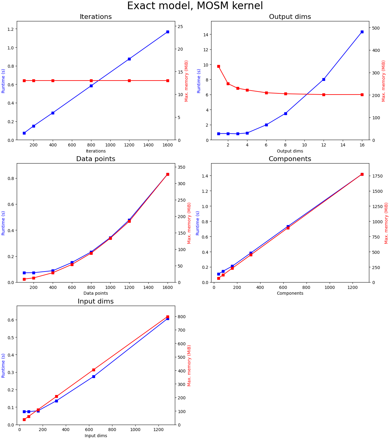
For each plot, we initialize a MOSM kernel and use exact inference (ie. without inducing points). The data is generated randomly of size (data_points,1+input_dims), where the first column contains the output indices. The output indices are assigned by dividing the data points in equal parts of output dimensions (ie. total number of data points is constant while we increase the number of output dimension). We keep the other four parameters constant while varying one parameter for each of the plots.
Conclusions:
- There are no memory leaks since memory is constant over iterations and time is linear
- It is quadratic over the number of data points, both in memory and time. I believe that Cholesky decomposition, which scales O(n^3), is really fast but that in this range the O(n^2) nature of the kernel matrix and other calculations is simply the slowest. For larger numbers of data points the cubic nature of time should take over.
- Both over the number of input dimensions and mixture components are linear in memory and time and are very fast in general. Note that these variables depend on the kernel and not on the inference model.
- It is quadratic in time but approximately O(1/n) for memory over the output dimensions. Both results are interesting. I believe that the sequential nature of how we compute each sub Gram matrix for each channel combination allows us to use less memory (which is recycled for each channel combination). Time is quadratic since we need to evaluate M*M sub Gram matrices, with M the number of channels.
Regarding the output dimensions, the sub Gram matrixes are of course smaller since the total number of data points is kept constant. However instead of using large vectorized operations as we'd have for a single output dimension, we have to process each sub kernel sequentially with smaller vectorized operations for each sub kernel. This can't be optimized further since the number of data points per channel is variable. When the number of data points for all channels is equal, we could write an optimized multi-output kernel that calculates the resulting Gram matrix at once instead of calculating all the sub Gram matrices.
Expand source code Browse git
"""
.. include:: ./documentation.md
"""
from .gpr.config import *
from .gpr.model import CholeskyException
from .util import *

from .transformer import *
from .data import *
from .dataset import *
from .init import *
from .model import *
from .models.sm import *
from .models.mosm import *
from .models.csm import *
from .models.sm_lmc import *
from .models.conv import *
from .models.mohsm import *
Sub-modules
mogptk.datamogptk.datasetmogptk.gprmogptk.initmogptk.modelmogptk.modelsmogptk.transformermogptk.util